1. Adversaries in Multiplicative Weights
Here’s some discussion about the issue of what the adverasary sees before it presents the cost vector. To begin, let’s remove the step where the algorithm actually makes a “prediction”. Instead, the algorithm only maintains a current weight vector 


where

There is no longer any randomization in the algorithm; it is completely deterministic.
Now, what is the adversary allowed to base the cost vector 

To examine the argument a bit more, consider the following adversaries:
- (Adversary Type 1) The adversary writes down a sequence of
cost vectors
up-front, and we run the (deterministic) MW algorithm on it. For each such sequence of cost vectors, and for each expert
, we have the guarantee that
where I’ve bundled all the additive terms into this “regret” term. - (Adversary Type 2) For each
, the adversary is “adaptive” but still deterministic: the new cost vector
So a Type 2 adversary is no more powerful than that of Type 1.
- (Adversary Type 3) For each
where the expectations is taken over the randomness of the adversary.The contrapositive of this statement says: if we have an adversary where the expected regret is high, there must be a fixed length-

![\displaystyle \sum_t \mathbb{E} [\overline{p}^{(t)} \cdot \overline{m}^{(t)}] \leq \sum_t \mathbb{E}[ {m}_i^{(t)}] + \text{regret}(T,\varepsilon,N). \ \ \ \ \ (2)](https://s0.wp.com/latex.php?latex=%5Cdisplaystyle++++%5Csum_t+%5Cmathbb%7BE%7D+%5B%5Coverline%7Bp%7D%5E%7B%28t%29%7D+%5Ccdot+%5Coverline%7Bm%7D%5E%7B%28t%29%7D%5D+%5Cleq+%5Csum_t+%5Cmathbb%7BE%7D%5B+++%7Bm%7D_i%5E%7B%28t%29%7D%5D+%2B+%5Ctext%7Bregret%7D%28T%2C%5Cvarepsilon%2CN%29.++++%5C+%5C+%5C+%5C+%5C+%282%29&bg=ffffff&fg=000000&s=0&c=20201002)
So you can indeed think of the adversary as choosing the cost vector
1.1. Predictions
Finally, what about the fact that the MW algorithm (as specified in lecture) was also making random predictions? The fact that the future decisions of the algorithm did not depend on these random predictions, and that the adversary does not see the prediction before it creates the cost vector, allows us to push the same argument through.
The easiest way to argue this may be to imagine that it’s not the algorithm that makes the predictions. The algorithm instead gives the vector 
2. John’s Example
John asked a good (and illustrative) question: what about the adversary looks at the current 


So the 


The saving grace is that even the best expert cannot have low cost: MW will ensure that all the experts will end up paying a non-trivial amount. Indeed, how does the vector

Then it moves to
And then to
After 

And so to

But you see the pattern: any fixed expert 

And what is our cost? Even if the weight vector

the expected cost using the cost vector 


So our

Assuming that 

So all is OK.
2.1. Another Example
But what if there were some hidden 


 subject to
 . But then the optimum value of the SDP is
  can take), but it not achieved by any feasible solution.
 for
for  . But the dual seeks to maximize
 . For symmetric (and hence for psd) matrices,
  .
. matrices
  , Tr(AB) = Tr(BA).
  .
.
 matrix
  ,
,  for all psd
  .
.  for which
  . But
. But  is psd, which shows that
  for some psd
  , defined by
  , is also psd. (This matrix
 such that
 ![{A_{ij} = E[a_ia_j]}](https://s0.wp.com/latex.php?latex=%7BA_%7Bij%7D+%3D+E%5Ba_ia_j%5D%7D&bg=ffffff&fg=000000&s=0&c=20201002) . Similarly, let
. Similarly, let ![{B_{ij} = E[b_ib_j]}](https://s0.wp.com/latex.php?latex=%7BB_%7Bij%7D+%3D+E%5Bb_ib_j%5D%7D&bg=ffffff&fg=000000&s=0&c=20201002) for r.v.s
for r.v.s  . Moreover, we can take the
  ‘s to be independent of the
  ‘s. So if we define the random variables
  , then
![\displaystyle C_{ij} = E[a_ia_j]E[b_ib_j] = E[a_ia_jb_ib_j] = E[c_i c_j],](https://s0.wp.com/latex.php?latex=%5Cdisplaystyle++C_%7Bij%7D+%3D+E%5Ba_ia_j%5DE%5Bb_ib_j%5D+%3D+E%5Ba_ia_jb_ib_j%5D+%3D+E%5Bc_i+c_j%5D%2C+&bg=ffffff&fg=000000&s=0&c=20201002)
 (i.e., it is positive definite),
  for all psd
  .
. where
where  is orthonormal, and
  is the diagonal matrix containing
  , and hence
  . Note that
  is psd: indeed,
  . So all of
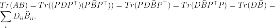
 and
and  for all
  for some
  if and only if
  .
. .
. ![{C_{ij} = E[c_ic_j]}](https://s0.wp.com/latex.php?latex=%7BC_%7Bij%7D+%3D+E%5Bc_ic_j%5D%7D&bg=ffffff&fg=000000&s=0&c=20201002) for random variables
for random variables  . Then
![\displaystyle A \bullet B = \sum_{ij} C_{ij} = \sum_{ij} E[c_ic_j] = E[\sum_{ij} c_ic_j] = E[(\sum_i c_i)^2].](https://s0.wp.com/latex.php?latex=%5Cdisplaystyle++A+%5Cbullet+B+%3D+%5Csum_%7Bij%7D+C_%7Bij%7D+%3D+%5Csum_%7Bij%7D+E%5Bc_ic_j%5D+%3D+E%5B%5Csum_%7Bij%7D+c_ic_j%5D+%3D+E%5B%28%5Csum_i+c_i%29%5E2%5D.+&bg=ffffff&fg=000000&s=0&c=20201002)
 must be zero with probability
 ![\displaystyle (AB)_{ij} = \sum_k E[a_ia_k]E[b_kb_j] = \sum_k E[a_ib_j(a_kb_k)] = E[a_ib_j (\sum_k c_k)] = 0,](https://s0.wp.com/latex.php?latex=%5Cdisplaystyle++%28AB%29_%7Bij%7D+%3D+%5Csum_k+E%5Ba_ia_k%5DE%5Bb_kb_j%5D+%3D+%5Csum_k+E%5Ba_ib_j%28a_kb_k%29%5D+%3D+E%5Ba_ib_j+%28%5Csum_k+c_k%29%5D+%3D+0%2C+&bg=ffffff&fg=000000&s=0&c=20201002)
 is identically zero.

 means we can find reals
  and unit vectors
  such that
  . By the fact that
  ‘s are unit vectors,
  , and the trace of this matrix is then
  . But by our constraints,
  , so
, so  .
. is the maximum of
 among these that maximizes
  ; that is at least as good as the average, right? Hence,
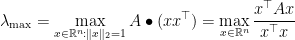
 either is basic (i.e., belongs to those four classes bip, co-bip, line(bip), or co-line(bip)), or else it has some structural “faults” (
 was not. Then

 . However, the LP solution given here (with
  on the thin edges, and
  on the thick ones) has
  . It also has
  , and you can check it satisfies the cut condition. (In fact, the main gadget that allows us to show this LP has an “integrality gap” is to assign
  to the edges of the thin triangle — much like for the naive non-bipartite matching LP.
 ) on that specially constructed directed graph gives an arborescence that corresponds to an integral maximum spanning tree on the original undirected graph.
 for
for  , and the constraints:
 of size at least
  and at most
  : if
: if  or
or  , then the first set of constraints already implies
  . So just focus on
 . We’ll call the first set of equalities the vertex constraints, and the second set the odd-set inequalities.
 (minimizing the sum of
  , say), and some vertex solution
  that is not integral. Clearly,
  must be even, else it will not satisfy the odd set constraint for
  . First, the claim is that
  cannot have a vertex of degree~
 , and neither being a cycle nor having a degree-
 . So
. So  .
. variables. So any vertex/BFS is defined by
  , then we could drop that edge
  and get a smaller counterexample. And since at most
  with
with  : i.e.,
 and
and  obtained by contracting
  and
and  to a single new vertex respectively, and removing the edges lying within the contracted set. Since both
  and
and  for these new graphs. E.g., to get
  for all edges
  . Note that if the set
  in
in  implies that
  , and hence
 is the natural vector representation of the perfect matching
  in
in  . Also,
  ‘s can be taken to be rational, since
 are perfect matchings in
  are rationals, we could have repeated the matchings and instead written

 ‘s are perfect matchings in
  , with
  . Note that
  . If we look at
  matchings
  matchings — contain
  ) up in the obvious way: apart from the edge
  , and
, and  . And
. And  . Hence putting together these perfect matchings
 , there is a matching
  that matches all the vertices on the left (i.e. has cardinality
  ) if and only if every set
  on the left has at least
  neighbors on the right. I wanted to point out that König’s theorem (which shows that the size of the maximum matching in
  ) is equivalent to Hall’s theorem. The proof is a fun exercise, so I’ll leave it out.
 , not just to
  .) Let’s go over these:
 . Then there exists an integer s-t cut
  with cost at most
  . (The proof was via the randomized rounding.) Note that this s-t cut corresponds to an integer vector
  where
where  , which is also feasible for the cut LP.
 is integral. To see this, consider any vertex
  . But since
  , and
, and  , it follows that
  and hence
  tight constraints? (Recall we were considering the LP
  ; since we were not talking about equational form LPs, the optimum could be achieved at a non-BFS.) He was right: we don’t. Here’s a proof.
 . Let
. Let  for
for  be all the constraints tight at
  generated by these vectors
  . If we prove this claim, we’re done–the rest of the argument follows that in lecture.
 such that
  for all
  . So now consider the point
  for some tiny
  . Note the following:
 . Consider
  for
for  : since this constraint was not tight, we won’t violate it if we choose
  small enough. And for
  ? See,
  , since
  .
.
 .
.
 . We didn’t quite answer is completely in class, here’s the complete explanation.
 ), or it is
  . Consider the LP obtained by adding in the new constraint
  . This is another equational form LP with
  constraints, and we can use the previous argument to decide feasibility. If this new LP is feasible, the original LP had optimum value