In case you hadn’t noticed, we’ve been trying to put up sample solutions for the HWs: complete solutions for HW2, and partial solutions for HW3 are now online (I still need to write the solutions for HW3 #1).
October 26, 2011
Homework Sample Solutions
October 26, 2011
Homework 2 graded
Homework 2 is graded. (Sorry for the delay, it’s my fault — AG). The average was (20/25). Some comments:
1. Most people got this, although in some cases with pretty long-winded proofs. The brief point is that when considering non-integral edges, every vertex on the V side has degree 0 or at least 2; thus one can find either a cycle (as in class) or else the maximal path starts and ends with a degree-1 vertex in U. Deepak cleverly pointed out that you can also just add |U|-|V| fictitious jobs called “unemployment”, link everyone to them with weight 0, and then reduce to the proof from class.
2. George & Leslie = Nemhauser & Trotter. Most people got this too, except in part (b) very few people observed out that for $x$ non-half-integral, $x^+$ and $x^-$ are distinct from $x$. Since this was really the only point to the question we should have deducted a point for failing to mention it. But we did not have the heart to do so.
3. Most people got the first 4 parts, and also the “easy” direction of Farkas Lemma (that both alternatives cannot be true). Some people had trouble with the last part (proving that if there is no feasible x then there must be a y): in particular, I saw proofs that tried to do it from first principles, where the hope was that you’d just use the template from the above parts (and use the correctness of the Avis-Kaluzny procedure).
4. This one tripped almost everyone up: very few of you even mentioned that one might not be able to reach the actual optimal LP value using binary search, and that some kind of “rounding” step would be needed at the end when the size of the binary search intervals is small enough. (That would have sufficed, since we didn’t really expect you to do this rounding step.) The details are all in the sample solutions: even if you don’t read all the solutions, have a look at this one for sure!
5. (Note: for this problem we should have stated that clauses always contain distinct literals. But this didn’t seem to trip anyone up.) Most everyone got (a) and (b). To some extent the point of this question was that for (c), the analysis is much easier than the proof that Horn-Sat is in P. All you have to do is say, “Given a solution with LP-value m, round each value down.” It’s very quick to check that the resulting integer solution still has value m.
October 24, 2011
Lecture 11: The Lovasz Theta Function
A draft of the lecture notes on SDPs and The Lovasz Theta Function have been posted.
October 22, 2011
No Lecture on Tuesday
In case you missed the announcement the other day, Tuesday October 25th’s lecture is canceled due to the FOCS conference. Normal service will resume on Thursday.
October 20, 2011
Lecture #12 (SDP duality): discussion
1. Examples
The example showing that the optimum value of an SDP might not be achieved is this: 

For this to be positive-semidefinite, we need 


Here is an example where the primal is feasible and finite, but the dual is infeasible.

The optimum is 

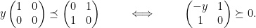
But this is infeasible, since psd matrices cannot have non-zero entries in the same row/column as a zero diagonal entry.
2. Proofs of Some Useful Facts
We used several facts about matrices in lecture today, without proof. Here are some of the proofs. Recall that 

 matrices
 Proof: 

Lemma 1 For a symmetric
matrix
,
for all psd
.
Proof:
One direction is easy: if 
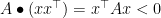


In the other direction, let 


by the definition of psd-ness of 
![{A_{ij} = E[a_ia_j]}](https://s0.wp.com/latex.php?latex=%7BA_%7Bij%7D+%3D+E%5Ba_ia_j%5D%7D&bg=ffffff&fg=000000&s=0&c=20201002)
![{B_{ij} = E[b_ib_j]}](https://s0.wp.com/latex.php?latex=%7BB_%7Bij%7D+%3D+E%5Bb_ib_j%5D%7D&bg=ffffff&fg=000000&s=0&c=20201002)


![\displaystyle C_{ij} = E[a_ia_j]E[b_ib_j] = E[a_ia_jb_ib_j] = E[c_i c_j],](https://s0.wp.com/latex.php?latex=%5Cdisplaystyle++C_%7Bij%7D+%3D+E%5Ba_ia_j%5DE%5Bb_ib_j%5D+%3D+E%5Ba_ia_jb_ib_j%5D+%3D+E%5Bc_i+c_j%5D%2C+&bg=ffffff&fg=000000&s=0&c=20201002)
and we are done. (Note we used independence of the
This clean random variable-based proof is from this blog post. One can also show the following claim. (I don’t know of a slick r.v. based proof—anyone see one?) BTW, the linear-algebraic proof also gives an alternate proof of the above Lemma 1.
Lemma 2 For
(i.e., it is positive definite),
for all psd
.
Proof: Let’s write 


Let 


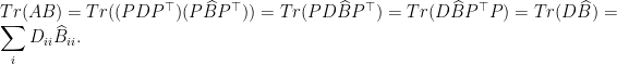
Since 


 if and only if
 Proof: Clearly if 

For the other direction, we use the ideas (and notation) from Lemma 1. Again take the Schur-Hadamard product ![{C_{ij} = E[c_ic_j]}](https://s0.wp.com/latex.php?latex=%7BC_%7Bij%7D+%3D+E%5Bc_ic_j%5D%7D&bg=ffffff&fg=000000&s=0&c=20201002)

![\displaystyle A \bullet B = \sum_{ij} C_{ij} = \sum_{ij} E[c_ic_j] = E[\sum_{ij} c_ic_j] = E[(\sum_i c_i)^2].](https://s0.wp.com/latex.php?latex=%5Cdisplaystyle++A+%5Cbullet+B+%3D+%5Csum_%7Bij%7D+C_%7Bij%7D+%3D+%5Csum_%7Bij%7D+E%5Bc_ic_j%5D+%3D+E%5B%5Csum_%7Bij%7D+c_ic_j%5D+%3D+E%5B%28%5Csum_i+c_i%29%5E2%5D.+&bg=ffffff&fg=000000&s=0&c=20201002)
If this quantity is zero, then the random variable 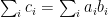

![\displaystyle (AB)_{ij} = \sum_k E[a_ia_k]E[b_kb_j] = \sum_k E[a_ib_j(a_kb_k)] = E[a_ib_j (\sum_k c_k)] = 0,](https://s0.wp.com/latex.php?latex=%5Cdisplaystyle++%28AB%29_%7Bij%7D+%3D+%5Csum_k+E%5Ba_ia_k%5DE%5Bb_kb_j%5D+%3D+%5Csum_k+E%5Ba_ib_j%28a_kb_k%29%5D+%3D+E%5Ba_ib_j+%28%5Csum_k+c_k%29%5D+%3D+0%2C+&bg=ffffff&fg=000000&s=0&c=20201002)
so 
3. Eigenvalues Seen Differently, or Old Friends Again
We saw that finding the maximum eigenvalue of a symmetric matrix

and its dual

The dual can be reinterpreted as follows: recall that 


Rewriting in this language, 

such that the 

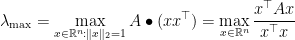
which is the standard variational definition of the maximum eigenvalue of
October 19, 2011
Lecture 10: Semidefinite Programs and the Max-Cut Problem
A draft of the lecture notes on semidefinite programs and the Max-Cut problem is posted.
October 19, 2011
Lecture 9: More on Ellipsoid: Grötschel-Lovász-Schrijver theorems
October 19, 2011
Homework #4 comments
There’ve been some corrections to homework 4, just in case you missed those.
Also, for the matroid problem (#2): if you’ve not seen matroids before, you might find it useful to think about the arguments in the special case of the graphical matroid first. In a graphical matroid, the elements are edges of some graph G, and the independent sets are all forests (acyclic subgraphs) of this graph.
October 18, 2011
Lecture #11 discussion
In the lecture, I forgot to mention why we chose to talk about the classes of perfect graphs we did. We showed that bipartite graphs and line graphs of bipartite graphs (and their complements) are all perfect.Let’s call a graph basic if it belongs to one of these four classes: bip, co-bip, line(bip), or co-line(bip).
Recall a graph was called a Berge graph if it did not contain (as an induced subgraph) any odd hole or odd antihole. Clearly, all perfect graphs are Berge graphs, else they could contain such a offending induced subgraph, which would contradict their perfectness. The other direction is the tricky one: showing that all Berge graphs are perfect. Which is what Maria Chudnovsky, Neil Robertson, Paul Seymour, and Robin Thomas eventually did in 2002.
So how did they proceed? Here’s a mile-high view of their approach. They showed that every Berge graph 
Re Srivatsan’s question: given the strong perfect graph theorem, the perfect graph theorem follows as a corollary. Indeed, suppose 
